Remote Sensing Lab Six: Geometric Correction

Background

Geometric correction is essential for accurately displaying an image because the way the data are collected do not indicate the correct X and Y location. This lab explored the two basic ways in how to correct an image so the data appear in the actual X and Y locations. Image to map rectification and Image to Image rectification were used. An image can only be rectified from a previously geometrically corrected image. So if many geometric corrections are needed to produce an outcome image then the original image used to correct a map/image MUST be already corrected for, otherwise the data points will still be in the wrong locations.


Methods

Image to Map Rectification

An AOI (area of interest) of the Chicago area was for the image to map rectification. In Erdas Imagine the Ground Control points are collected using the Multipoint Geometric Correction window.

After adding the reference image and map image into two separate viewers, click the multispectral tab and then "Control Points".

The Geometric Model was set to Polynomial since that was the desired model to employ. In the GCP Tool Reference Setup select "New Layer". Enter the imput DRG (Digital Raster Graphic) for the reference image and accept the default "Polynomial Model Properties".

Now it is possible to start collecting GCP's (Ground Control Points) in the Multipoint Geometric Correction window. Since we selected a first order polynomial model, a minimum of three GCP's have to be collected.

To do this select the "Create GCP" tool and add a GCP to the map and the reference image. The properties of the GCP (i.e. color) can be changed in the panel at the bottom. Repeat twice more to fulfill the requirements of the first order polynomial. When the minimum number of GCP points is reached for a  polynomial model the model solution changes to "Model solution is current". Now, GCP's will only be added to one image and the program will automatically place a GCP in the complementary location on the other image.

To reduce the root mean square error (RMS) after all the GCP's have been collected, zoom into the first GCP more. Move the GCP so that the total RMS (in the bottom right corner) decreases a little. Then, proceed the same process with the rest of the GCP's until the RMS error is below 2.

When the RMS error is satisfied then the "Display Resample Image" tool at the top of the Multipoint Geometric Correction tool bar. Save the output image to a personal folder and bring the image into Erdas to view the final product.


Image to Image Rectification

Image to Image Rectification is done by the same process with the image to map rectification above. For this part of the lab, the images were from Sierra Leone, Africa.

A big difference from the directions above is that for this example a third order polynomial was used which requires ten ground control points, instead of the three we needed before.

Finally, with all the GCP's collected and with a total RMS error of less than 1 the "Display Resample Image" tool was used again.

Results

Figure 1. Image to Map rectification using Erdas Imagine. The ground control points are displayed white on the reference image and purple on the map. An RMS of less than 2 was achieved. 

Figure 2. Image to Image Rectification. The ground control points are displayed yellow in both images. An RMS of 0.97 was achieved. 

The rectified images showed great improvement from the originals. It is now possible to analyze the rectified image with confidence that the X and Y locations are verified and true to the same location on the Earth.

Conclusion

In conclusion, geometric correction is crucial in creating a spatially accurate representation of the actual locations of the Earth's features. Omitting this process as part of image analysis would seriously alter the results and could have great repercussions. It is important to understand geometric correction, the polynomial model, and RMS error in order to produce proper images.


Sources
Satellite images
Earth Resources Observation and Science Center, United States Geological Survey

Digital raster graphic (DRG)
Illinois Geospatial Data Clearing House

Remote Sensing Lab 5: LiDAR Remote Sensing

Background

LiDAR data collection and utilization have become very popular and increasing useful recently in the field of remote sensing. LiDAR can be used across many disciplines and is helpful for data analysis.

Objectives/Goals

• To produce surface and terrain models
• To create an intensity image and other rasters (DSM and DTM) from a point cloud dataset (LAS format) 

Methods

Making surface and terrain models

1. Copy the LAS files into a personal folder and create a new LAS Dataset
2. Add the LAS files into the LAS dataset by clicking the "Add Files" button and selecting ALL the LAS file in the folder
3. Examine the LAS files to see if the files are already assigned a coordinate system
4. If the data files did not have a predefined coordinate system, look to the metadata to choose the correct CS
5. In the Dataset properties set the X,Y Coordinate System and Z Coordinate System to the correct selections

(Since we were handling data from Eau Claire the X,Y Coordinate System was set to NAD 1983 HARN Wisconsin CRS Eau Claire (US Feet) and the Z-Coordinate System to NAVD 1988 US feet)

We added the LAS dataset to ArcMap and a grid appeared. Only if the map was zoomed in could we see the specific points. Before continuing, a shapefile of Eau Claire was added to ensure the correct location of the dataset. This is recommended for checking to see if an appropriate coordinate system is in place.

6. Turn on the LAS Dataset toolbar in ArcMap! (To do this the 3-D analyst extension from the Customize toolbar has to be active)

7. By selecting different options from the LAS dataset toolbar it is possible to explore various types of surface/terrain models from the point cloud. See Figure 1 below.

Figure 1. The LAS Dataset toolbar in ArcMap allows to to change how to view the points from the LAS files. 

The tool highlighted (blue box) from the LAS Dataset toolbar in Figure 1. above is the Point Symbology Renders. The dropdown box allows the user to choose: elevation, class, or return. This determines how the points will be displayed (based on the elevation, based on their classification code, or based on the lidar pulse return number).

The surface symbology render options are elevation, aspect, slope, and countour. See Figure 2. to compare the differences in these displays.

Figure 2. LAS surface symbology renders from a section of Eau Claire County, Wisconsin. 

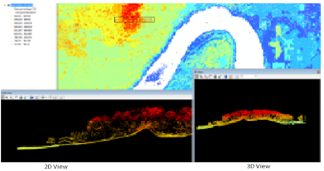
The tool not available in Figure 1. LAS Dataset Profile View allows the user to view the lidar point cloud data in a 2-D view. A pop-up screen will appear.

Finally, the LAS Dataset 3-D view is available to view the lidar data as well. This is helpful in viewing the Z aspect of the image.

Figure 3. 2D and 3D views form the Eau Claire County, Wisconsin lidar point cloud dataset. 

Creating an intensity image

In this section of the lab we focused on creating DSM and DTM models of the point cloud lidar data.

Average Nominal Pulse Spacing is crucial in figuring out what the spatial resolution should be for  the DSM and DTM output images.

a) Digital surface model (DSM) with first return 

First, set the lidar points to elevation and filter to First Return. This way the image will only show the elevation of the first pulse sent back to the sensor.

Next, use the LAS Dataset to Raster tool (Conversion --> Raster) to create the DSM.

The LAS Dataset to Raster window will appear and fill in the appropriate values for your desired outcome. The value field was set to elevation. The interpolation settings were binning, maximum, and nearest neighbor. Since our data was 2 meters by 2 meters we set the sampling value to 6.56168 (roughly 2m in feet). All the other values were set to default.

***Important: when naming the output file to a personal folder make sure to add .TIF at the end to save the rasters in the TIFF format. This allows you to open the images in Erdas after.

b) Digital terrain model (DTM)

To create the DTM the same steps as above were carried out through the LAS Dataset to Raster tool, expect before the elevation and ground filter were used for the dataset. In this case we specifically used the binning interpolation method again but selected minimum and nearest neighbor as the settings. All other settings were the same as in creating the DSM. Again, do not forget to add the .TIF to the end of the output file name.


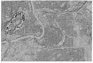
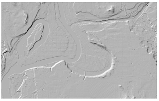
c) Hillshade of  DSM and DTM

The next step was to hillshade the DSM and DTM. To do this it was necessary to use the Hillshade tool in the 3D Analyst toolbox under Raster Surfacing. The pop-up window was easy to navigate, entering in the input rasters created above. Save these outputs as .TIF files as well.

Figure 4. Hillshade output from DSM. 

Figure 5. HIllshade output from DTM. 

d) Intensity Image 

The Dataset to Raster tool was used again to create the intensity image, however, the point cloud data was set to Return for the Point Symbology and the filter was set to First Return. The value field should be set to INTENSITY and the interpolation should be set to binning (average and nearest neighbor). The 6.56168 value was entered again as the sampling value.

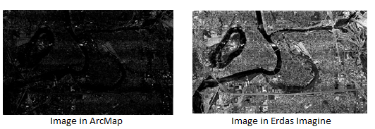
After the raster was created in ArcMap, the image appeared very dark. It was difficult to distinguish features. But,  if viewed in Erdas Imagine the image was much brighter and easy to interpret. See Figure 4. below. To import the image into Erdas Imagine the file needs to be saved in the .TIF format.

Figure 4. Intensity image produced from the Dataset to Raster tool displayed in ArcMap vs. Erdas Imagine. 

Conclusion

Knowing how to correctly use and analyze raster data is the foundation to remote sensing. LiDAR data is becoming more and more accessible and being able to effectively manipulate the data can open up so many possibilities across many disciplines. This lab allowed us to get a taste of experimenting with point cloud lidar data and understand some of the challenges it presents us with if not done correctly.

Sources

Lidar point cloud and Tile Index
Eau Claire County, 2013. Eau Claire County Shapefile is from Mastering ArcGIS 6th Edition data by Margaret Price, 2014.